TL;DR

The distance-preserving property of random projections discovered in 1984 (the JL Lemma) becomes, 40 years later, the central tool for compressing the KV Cache of LLMs to its limits. Following the research arc from QJL (2024) → PolarQuant (2025) → TurboQuant (2025), we arrive at the theoretical conclusion that "a single random rotation is enough for optimal quantization." In practice, however, the QJL residual correction — supposedly the centerpiece of the theory — can actually hurt, and there is an ongoing academic dispute about the relationship to prior work (RaBitQ).

Figure 1. Forty years of research, from the JL Lemma (1984) to TurboQuant (2025).

The KV Cache Problem

Anyone who has served LLMs knows that for long-context inference, the real bottleneck is not the model weights but the KV Cache. Every time a Transformer generates a token, it has to keep the Key-Value embeddings of every previous token in memory.

The attention score [25] makes this immediately clear (we omit the \(1/\sqrt{d_{k}}\) scaling for brevity):

\[\text{Score}=\text{softmax} \big( [\langle q_{n},k_{1}\rangle ,\langle q_{n},k_{2}\rangle ,\ldots ,\langle q_{n},k_{n}\rangle ] \big)\]

Here \(q_{n}\) is the current query, and \(k_{1},\ldots ,k_{n}\) are the cached key embeddings. The inner product \(\langle q_{n},k_{i}\rangle\) measures "how relevant is the \(i\)-th past token to the current question?" As the conversation grows, the number of keys we have to refer to grows linearly, and so does the KV Cache.

The scale of the problem is clearer with concrete numbers.

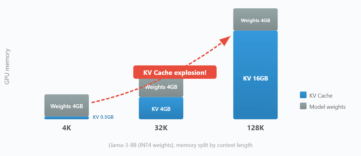
Figure 2. As the context grows, the KV Cache dwarfs the model weights. At 128K, it's 4× larger.

If you quantize Llama-3-8B's weights to INT4, they take about 4 GB. But processing a 128K context blows the KV Cache up to 16 GB or more — four times the model weights. (Rough estimate for a single sequence with FP16 KV: 32 layers × 8 KV heads × 128 head_dim × 2(K+V) × 2 bytes × 128K tokens.) GPTQ, AWQ, and friends shrink the weights as much as you like, but if you ignore the KV Cache, none of it matters.

Quantization Overhead Problem

Naturally, people have tried to quantize the KV Cache too. KIVI [23] assigns asymmetric bit widths to keys and values (2-bit per-channel for keys, 2-bit per-token for values) and pushes down to 2 bits without any tuning. KVQuant [24] adds outlier separation, non-uniform codebooks, and dense-and-sparse decomposition on top, targeting ultra-long contexts in the 10M-token range. Both methods share a common pattern: they split the data into blocks and store an auxiliary scale and zero-point for each block.

The catch is that these auxiliary constants cost more than you'd think. With FP16 storage:

• Group size 128 + 4-bit quantization: 128 × 4 bits + 16 bits (scale) + 16 bits (zero) = 544 bits, effectively 4.25 bits/value

• Group size 32 + 4-bit quantization: 32 × 4 bits + 32 bits = 160 bits, effectively 5 bits/value

With FP32 storage the overhead is even bigger, climbing to roughly 6 bits/value at group size 32.

Smaller groups give better quality but the overhead keeps growing, and what was supposed to be "4-bit quantization" actually uses 6 bits in practice. QJL, PolarQuant, and TurboQuant — the methods we'll cover in this post — all try to eliminate this overhead at the root, and it's a bit surprising that the starting point is pure mathematics from 1984.

Distance Preservation in Random Projections

The Johnson-Lindenstrauss Lemma

What Johnson and Lindenstrauss [20] discovered in 1984 sounds counterintuitive at first: if you project high-dimensional vectors randomly down to a lower dimension, the pairwise distances between points are preserved almost exactly.

The Heart of the JL Lemma (Lemma 1.1 [1])

Randomly project points in \(\mathbb{R}^{d}\) down to \(\mathbb{R}^{m}\), and all pairwise distances are preserved up to a factor of \((1\pm \epsilon )\). The crucial point is that the required target dimension \(m=O(\epsilon ^{-2}\log n)\) does not depend on the original dimension \(d\) at all.

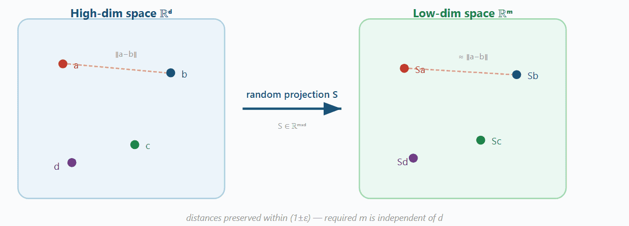
Figure 3. The intuition behind the JL Lemma: a random projection nearly preserves the distances between points.

Whether you start with a million-dimensional vector or a billion-dimensional one, preserving pairwise distances of \(n\) points to within 10% only requires \(m\approx 100\cdot \log n\) dimensions. Concretely, if we define the JL transform as \(f(x)=\frac{1}{\sqrt{m}}Sx\) (where each entry of \(S\in \mathbb{R}^{m\times d}\) is i.i.d. \(N(0,1)\) [1][21]), the distributional JL Lemma (Lemma 1.2 [1]) guarantees:

\[\Pr \big[ | \|f(x)\|_{2}^{2}-\|x\|_{2}^{2} | >\epsilon \|x\|_{2}^{2} \big] \le \delta \text{when }m=O(\epsilon ^{-2}\log (1/\delta ))\]

The \(\frac{1}{\sqrt{m}}\) normalization is what makes this work: if \(S_{ij}\sim N(0,1)\) then \(\mathbb{E}[\|Sx\|^{2}]=m\|x\|^{2}\), so we need to multiply by \(\frac{1}{\sqrt{m}}\) for \(\mathbb{E}[\|f(x)\|^{2}]=\|x\|^{2}\) to hold. (QJL [2] absorbs this normalization into the \(1/m\) factor of its estimator instead of into \(S\) itself.)

Since lengths are preserved, inner products (Corollary 1.5 [1]) follow immediately:

\[| \langle f(x),f(y)\rangle -\langle x,y\rangle | \le \epsilon \|x\|_{2}\|y\|_{2}\]

Given that attention itself is just a stack of inner products, it should be obvious why this property matters. (The proof comes from the polarization identity \(4\langle u,v\rangle =\|u+v\|^{2}-\|u-v\|^{2}\) [1].)

Sanity check: does a JL projection preserve distances?

import numpy as np
d, m, n = 1000, 50, 200  # 1000 dims → 50 dims, 200 vectors
X = np.random.randn(n, d)
S = np.random.randn(m, d) / np.sqrt(m)  # 1/√m normalization
X_proj = (S @ X.T).T

# Compare pairwise distances in original vs projected space
i, j = 0, 1
dist_orig = np.linalg.norm(X[i] - X[j])
dist_proj = np.linalg.norm(X_proj[i] - X_proj[j])
print(f"original: {dist_orig:.3f}, projected: {dist_proj:.3f}, ratio: {dist_proj/dist_orig:.3f}")
# → ratio close to 1 (even when shrinking 1000 dims down to 50!)

import numpy as np
d, m, n = 1000, 50, 200  # 1000 dims → 50 dims, 200 vectors
X = np.random.randn(n, d)
S = np.random.randn(m, d) / np.sqrt(m)  # 1/√m normalization
X_proj = (S @ X.T).T

# Compare pairwise distances in original vs projected space
i, j = 0, 1
dist_orig = np.linalg.norm(X[i] - X[j])
dist_proj = np.linalg.norm(X_proj[i] - X_proj[j])
print(f"original: {dist_orig:.3f}, projected: {dist_proj:.3f}, ratio: {dist_proj/dist_orig:.3f}")
# → ratio close to 1 (even when shrinking 1000 dims down to 50!)

import numpy as np
d, m, n = 1000, 50, 200  # 1000 dims → 50 dims, 200 vectors
X = np.random.randn(n, d)
S = np.random.randn(m, d) / np.sqrt(m)  # 1/√m normalization
X_proj = (S @ X.T).T

# Compare pairwise distances in original vs projected space
i, j = 0, 1
dist_orig = np.linalg.norm(X[i] - X[j])
dist_proj = np.linalg.norm(X_proj[i] - X_proj[j])
print(f"original: {dist_orig:.3f}, projected: {dist_proj:.3f}, ratio: {dist_proj/dist_orig:.3f}")
# → ratio close to 1 (even when shrinking 1000 dims down to 50!)

How JL Matrices Evolved

The random matrix realizing the JL transform (the JL distribution) has steadily evolved over four decades [1]. Early constructions filled the entire matrix with Gaussian \(N(0,1)\) [21] or Rademacher \(\pm 1\) entries (the Dense construction, \(O(md)\) time). Achlioptas [22] then proposed a Sparse construction zeroing out 2/3 of the entries. The reason sparsity works is interesting: if a vector's \(\ell _{\infty }/\ell _{2}\) ratio is small — that is, its energy is spread evenly rather than concentrated on a few coordinates — you can fill most of the matrix with zeros and still preserve distances (Theorem 1.8 [1]). Finally, Ailon and Chazelle [17] turned this observation into a structural one with the FFT-based construction (FJLT): first reduce \(\ell _{\infty }/\ell _{2}\) using a Hadamard transform, then project with a sparse matrix.

The key piece is Ailon and Chazelle's Fast JL Transform (FJLT) [17]:

\[f(x)=P\cdot H\cdot D\cdot x\]

Each of the three matrices plays a specific role:

\(D\): a diagonal Rademacher matrix — \(+1\) or \(-1\) with equal probability on the diagonal. Multiplying a vector by it randomly flips the sign of each coordinate. For example, with \(d=4\):

\[D= \Big( \begin{array}{cccc}+1&0&0&0\\ 0&-1&0&0\\ 0&0&+1&0\\ 0&0&0&-1\end{array} \Big) ,D \Big( \begin{array}{c}3\\ 7\\ 2\\ 5\end{array} \Big) = \Big( \begin{array}{c}3\\ -7\\ 2\\ -5\end{array} \Big)\]

The point of this stage is that, even if the input vector has its energy concentrated on a few coordinates, mixing the signs prepares it so the next stage (Hadamard) can spread the energy out evenly.

\(H\): the Walsh-Hadamard matrix — an orthogonal matrix consisting only of \(\pm 1\), defined recursively:

\[H_{1}=(1),H_{2}=\frac{1}{\sqrt{2}} \bigg( \begin{array}{cc}1&1\\ 1&-1\end{array} \bigg) ,H_{4}=\frac{1}{2} \Big( \begin{array}{cccc}1&1&1&1\\ 1&-1&1&-1\\ 1&1&-1&-1\\ 1&-1&-1&1\end{array} \Big)\]

Multiplying a vector by \(H\) takes every additive/subtractive combination of its coordinates, so even a vector with its energy concentrated in one coordinate gets spread evenly across all of them. The key point is that, thanks to a butterfly structure like the FFT's, this can be computed in \(O(d\log d)\), and since it only uses \(\pm 1\), it requires no multiplications at all — particularly attractive for hardware accelerators like NPUs.

\(P\): a sparse projection matrix — an \(m\times d\) matrix with mostly zero entries that reduces the dimension from \(d\) to \(m\). After the \(HD\) stage the vector's energy is already spread evenly, so a sparse matrix is enough for a good projection [1]. For instance, with \(d=4,m=2\):

\[P= \bigg( \begin{array}{cccc}0&1.2&0&0\\ 0&0&0&-0.8\end{array} \bigg)\]

Combining these three stages: \(D\) mixes the signs, \(H\) spreads the energy, and \(P\) reduces the dimension. The total time is dominated by \(H\)'s \(O(d\log d)\), much faster than the dense construction's \(O(md)\). QJL, PolarQuant, and TurboQuant — which we'll see below — all use the \(HD\) stage of FJLT (random sign flips + Hadamard transform) as a core preprocessing step. The difference is that they apply quantization in place of the \(P\) (dimension reduction) step.

Sanity check: does Hadamard spread out the energy?

import numpy as np
from scipy.linalg import hadamard
d = 128
H = hadamard(d) / np.sqrt(d)       # normalized Hadamard (d must be a power of 2)
D = np.diag(np.random.choice([-1, 1], d))  # random signs

x = np.zeros(d); x[0] = 1.0      # energy concentrated in one coordinate
y = H @ D @ x                      # HD transform
print(f"max/norm before: {np.max(np.abs(x)):.3f}")   # → 1.000
print(f"max/norm after:  {np.max(np.abs(y)):.3f}")   # → 0.088 (energy spread!)

import numpy as np
from scipy.linalg import hadamard
d = 128
H = hadamard(d) / np.sqrt(d)       # normalized Hadamard (d must be a power of 2)
D = np.diag(np.random.choice([-1, 1], d))  # random signs

x = np.zeros(d); x[0] = 1.0      # energy concentrated in one coordinate
y = H @ D @ x                      # HD transform
print(f"max/norm before: {np.max(np.abs(x)):.3f}")   # → 1.000
print(f"max/norm after:  {np.max(np.abs(y)):.3f}")   # → 0.088 (energy spread!)

import numpy as np
from scipy.linalg import hadamard
d = 128
H = hadamard(d) / np.sqrt(d)       # normalized Hadamard (d must be a power of 2)
D = np.diag(np.random.choice([-1, 1], d))  # random signs

x = np.zeros(d); x[0] = 1.0      # energy concentrated in one coordinate
y = H @ D @ x                      # HD transform
print(f"max/norm before: {np.max(np.abs(x)):.3f}")   # → 1.000
print(f"max/norm after:  {np.max(np.abs(y)):.3f}")   # → 0.088 (energy spread!)

Connection to Deep Learning Quantization

The connection between this 40-year-old theory and KV Cache compression has three threads.

First, the motivation of energy spreading is the same. SmoothQuant [6] uses diagonal scaling to spread out outliers; QuIP [18] and QuIP# [19] use Hadamard rotations directly. The methods differ (SmoothQuant uses a data-dependent diagonal matrix, FJLT uses a random Rademacher + Hadamard) but the goal is identical: take energy concentrated on a few channels and spread it across all dimensions so uniform quantization can do its job efficiently.

Second, preserving inner products is a key precondition for accuracy. Neural network inference is a chain of matrix multiplications (\(y=Wx\)), and if quantization preserves inner products (JL Corollary 1.5 [1]) the output of each individual linear operation is preserved. That said, once you go through nonlinear operations like softmax or layernorm, preserving inner products is no longer enough to guarantee final accuracy — we'll come back to this limitation in section 7.

Third, the \(\ell _{\infty }/\ell _{2}\) ratio is a measure of quantization efficiency. This ratio captures "how concentrated is a vector's energy on a single coordinate" (Theorem 1.8 [1]). The smaller the ratio — the more evenly the energy is spread — the more efficient a uniform quantization grid becomes, and the fewer bits you need. This observation explains the core strategy of existing quantization methods:

• SmoothQuant [6] uses diagonal scaling to migrate outliers from activations to weights, reducing the activations' \(\ell _{\infty }/\ell _{2}\) ratio. It's data-dependent (calibration is needed) and still uses standard uniform quantization (scale + zero-point) after the transform.

• SpinQuant [7] learns an orthogonal rotation that flattens the distribution. It still applies standard uniform quantization after the rotation, so the per-group scale/zero-point overhead remains.

• The TurboQuant family [2][3][4] that we'll see below goes a step further: rather than just reducing the \(\ell _{\infty }/\ell _{2}\) ratio with a random rotation, they exploit the fact that the post-rotation distribution is analytically predictable to design the quantizer optimally without any data. There's no overhead at all.

Now let's see how these tools actually get used to compress the KV Cache.

QJL: Inner Product Recovery from a Single Sign Bit

Asymmetric Quantization — Only Keys to 1-bit

In a KV Cache, keys live in memory until the conversation ends, but queries are only used for the current token's generation and then discarded. QJL [2] exploits this asymmetry: it projects both keys and queries through the same random matrix \(S\), but for keys it stores only the sign bits of the projection, while for queries it keeps the projection at full precision. Only the keys live in the cache, so only the keys get extreme compression — an asymmetric design.

Figure 4. The asymmetric QJL pipeline. Keys are squeezed down to 1 bit, queries stay at full precision.

The inner-product estimator is:

\[\hat{\langle q,k\rangle }=\frac{\sqrt{\pi /2}}{m}\cdot \|k\|_{2}\cdot \langle Sq,\text{sign}(Sk)\rangle\]

Why a Single Sign Bit Recovers the Inner Product

This is the part of the paper I found most striking, and the unbiasedness proof is cleaner than you'd expect. It comes in four steps.

Decompose. Split the query \(q\) into components parallel and perpendicular to the key \(k\): \(q=\frac{\langle q,k\rangle }{\|k\|^{2}}k+q_{k}^{\perp }\).

Expand. For each row \(s_{i}\), using \(x\cdot \text{sign}(x)=|x|\):

\[s_{i}^{\top }q\cdot \text{sign}(s_{i}^{\top }k)=\frac{\langle q,k\rangle }{\|k\|^{2}}\cdot |s_{i}^{\top }k|+s_{i}^{\top }q_{k}^{\perp }\cdot \text{sign}(s_{i}^{\top }k)\]

Take expectation. The perpendicular component just vanishes — because \(k\) and \(q_{k}^{\perp }\) are orthogonal, the projections of a Gaussian vector \(s_{i}\) onto each, \(s_{i}^{\top }k\) and \(s_{i}^{\top }q_{k}^{\perp }\), are independent (for Gaussians, uncorrelated implies independent [2]). So the expectation of the product is zero. On the parallel side, Step 2 turned things into \(s_{i}^{\top }k\cdot \text{sign}(s_{i}^{\top }k)=|s_{i}^{\top }k|\). Since \(s_{i}\) is Gaussian, \(s_{i}^{\top }k\sim N(0,\|k\|^{2})\), and the expected absolute value of this normal distribution is \(\mathbb{E}[|x|]=\|k\|\cdot \sqrt{2/\pi }\) (the mean of what's called the half-normal distribution).

Cancellation. Returning to the definition of the estimator and expanding the expectation: by Step 3 the perpendicular part is gone, leaving only the parallel part.

\[\mathbb{E} \Bigg[ \frac{\sqrt{\pi /2}}{m}\|k\|\sum_{i=1}^{m}(s_{i}^{\top }q)\cdot \text{sign}(s_{i}^{\top }k) \Bigg] =\frac{\sqrt{\pi /2}}{m}\|k\|\sum_{i=1}^{m}\frac{\langle q,k\rangle }{\|k\|^{2}}\cdot \mathbb{E}[|s_{i}^{\top }k|]\]

Substituting \(\mathbb{E}[|s_{i}^{\top }k|]=\|k\|\sqrt{2/\pi }\) from Step 3 and dividing the sum of \(m\) terms by \(m\), we are left with a single term:

\[=\sqrt{\frac{\pi }{2}}\cdot \|k\|\cdot \frac{\langle q,k\rangle }{\|k\|^{2}}\cdot \|k\|\cdot \sqrt{\frac{2}{\pi }}=\sqrt{\frac{\pi }{2}}\cdot \sqrt{\frac{2}{\pi }}\cdot \langle q,k\rangle =1\cdot \langle q,k\rangle =\langle q,k\rangle\]

In the end, the correction factor \(\sqrt{\pi /2}\) is chosen specifically to exactly cancel the \(\sqrt{2/\pi }\) coming from the half-normal.

QJL estimator behavior

import numpy as np
d, m = 128, 4096  # larger m → smaller variance
q = np.random.randn(d); q /= np.linalg.norm(q)  # unit norm
k = np.random.randn(d); k /= np.linalg.norm(k)
S = np.random.randn(m, d)

# QJL estimator: store only sign(Sk), keep Sq at full precision
sign_Sk = np.sign(S @ k)
estimate = np.sqrt(np.pi/2) / m * np.linalg.norm(k) * (S @ q) @ sign_Sk

print(f"true inner product: {q @ k:.4f}")
print(f"QJL estimate:       {estimate:.4f}")  # → single trial (variance scales as ‖q‖‖k‖/√m)
# To verify unbiasedness directly, average across many S

import numpy as np
d, m = 128, 4096  # larger m → smaller variance
q = np.random.randn(d); q /= np.linalg.norm(q)  # unit norm
k = np.random.randn(d); k /= np.linalg.norm(k)
S = np.random.randn(m, d)

# QJL estimator: store only sign(Sk), keep Sq at full precision
sign_Sk = np.sign(S @ k)
estimate = np.sqrt(np.pi/2) / m * np.linalg.norm(k) * (S @ q) @ sign_Sk

print(f"true inner product: {q @ k:.4f}")
print(f"QJL estimate:       {estimate:.4f}")  # → single trial (variance scales as ‖q‖‖k‖/√m)
# To verify unbiasedness directly, average across many S

import numpy as np
d, m = 128, 4096  # larger m → smaller variance
q = np.random.randn(d); q /= np.linalg.norm(q)  # unit norm
k = np.random.randn(d); k /= np.linalg.norm(k)
S = np.random.randn(m, d)

# QJL estimator: store only sign(Sk), keep Sq at full precision
sign_Sk = np.sign(S @ k)
estimate = np.sqrt(np.pi/2) / m * np.linalg.norm(k) * (S @ q) @ sign_Sk

print(f"true inner product: {q @ k:.4f}")
print(f"QJL estimate:       {estimate:.4f}")  # → single trial (variance scales as ‖q‖‖k‖/√m)
# To verify unbiasedness directly, average across many S

Figure 5. The geometric intuition for sign bits. Random hyperplanes partition space, and the fraction of times \(k\) and \(q\) end up on the same side encodes the inner product.

Geometrically, a sign bit encodes "which side of a random hyperplane is this vector on?" Two vectors pointing in similar directions land on the same side of most hyperplanes; near-orthogonal vectors split roughly fifty-fifty. This "fraction of same-side" determines the inner product.

QJL's storage layout is also worth noting. Per token, you only need \(m\) sign bits plus 16 bits for the norm, with no per-group scale or zero-point. The scale/zero-point overhead from section 1 is gone.

QJL is a nice idea, but it has one fundamental limitation: you can't reconstruct the original vector. With sign bits alone you can estimate inner products, but you can't bring back the vector itself, which means it's useless for the value (V) cache. The value cache needs to compute weighted sums of the actual vectors, not inner products. How do we get past this?

PolarQuant: A Different Coordinate System

Why Convert to Polar Coordinates

PolarQuant [3] takes a different angle: change the coordinate system. It converts KV embeddings from Cartesian to polar coordinates (radius + angles) and quantizes the angles. Just as latitude is always in \([-90°,90°]\), the angles in polar coordinates have fixed ranges, so no data-dependent scale or zero-point is needed.

The Recursive Polar Transform

Converting a 128-dimensional vector to polar coordinates all at once gives you 127 angles tangled together in messy ways. PolarQuant solves this recursively:

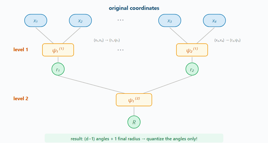
Figure 6. PolarQuant's recursive polar transform (4-dimensional example). Coordinates are paired up and the 2D polar transform is applied repeatedly.

1. Pair up coordinates and apply a 2D polar transform: \((x_{2j-1},x_{2j})\mapsto (r_{j},\psi _{j})\).

2. Pair up the resulting radii \(r_{1},r_{2},\ldots\) and repeat.

3. After \(\log_{2}d\) iterations you end up with \(d-1\) angles and one final radius.

The core of the recursive polar transform

import numpy as np

def recursive_polar(x):
    """Pair up coordinates as (radius, angle) and recurse on the radii.
    The length of x must be a power of 2."""
    angles, radii = [], []
    for i in range(0, len(x), 2):
        r = np.sqrt(x[i]**2 + x[i+1]**2)
        psi = np.arctan2(x[i+1], x[i])
        radii.append(r); angles.append(psi)
    if len(radii) > 1:
        deeper_angles, final_r = recursive_polar(np.array(radii))
        return angles + deeper_angles, final_r
    return angles, radii[0]

# 8-dimensional vector → 7 angles + 1 radius
x = np.random.randn(8); x /= np.linalg.norm(x)
angles, r = recursive_polar(x)
print(f"{len(angles)} angles + radius {r:.4f}")  # → 7 angles + 1.0000

import numpy as np

def recursive_polar(x):
    """Pair up coordinates as (radius, angle) and recurse on the radii.
    The length of x must be a power of 2."""
    angles, radii = [], []
    for i in range(0, len(x), 2):
        r = np.sqrt(x[i]**2 + x[i+1]**2)
        psi = np.arctan2(x[i+1], x[i])
        radii.append(r); angles.append(psi)
    if len(radii) > 1:
        deeper_angles, final_r = recursive_polar(np.array(radii))
        return angles + deeper_angles, final_r
    return angles, radii[0]

# 8-dimensional vector → 7 angles + 1 radius
x = np.random.randn(8); x /= np.linalg.norm(x)
angles, r = recursive_polar(x)
print(f"{len(angles)} angles + radius {r:.4f}")  # → 7 angles + 1.0000

import numpy as np

def recursive_polar(x):
    """Pair up coordinates as (radius, angle) and recurse on the radii.
    The length of x must be a power of 2."""
    angles, radii = [], []
    for i in range(0, len(x), 2):
        r = np.sqrt(x[i]**2 + x[i+1]**2)
        psi = np.arctan2(x[i+1], x[i])
        radii.append(r); angles.append(psi)
    if len(radii) > 1:
        deeper_angles, final_r = recursive_polar(np.array(radii))
        return angles + deeper_angles, final_r
    return angles, radii[0]

# 8-dimensional vector → 7 angles + 1 radius
x = np.random.randn(8); x /= np.linalg.norm(x)
angles, r = recursive_polar(x)
print(f"{len(angles)} angles + radius {r:.4f}")  # → 7 angles + 1.0000

Distribution of Angles After Rotation

The key mathematical insight is here. After multiplying by a random rotation matrix \(S\), the distribution of the angles at each level \(\ell\) takes an analytically known form:

\[f_{\Psi ^{(\ell )}}(\psi )\propto \sin^{2^{\ell -1}-1}(2\psi )\]

Figure 7. Angle distributions by level. Higher levels concentrate sharply around \(\pi /4\), so they can be quantized with fewer bits.

As the level grows, the distribution concentrates ever more sharply around \(\pi /4\). This enables an efficient bit budget: 4 bits at the first level (a wide distribution that needs fine quantization), 2 bits per level for the rest (concentrated distributions where fewer bits suffice).

Where PolarQuant Improves on QJL

PolarQuant has two main advantages over QJL.

First, you can reconstruct the original vector. From the quantized angle \(\hat{\psi }\) and the radius \(r\), the standard polar inverse transform recovers the Cartesian coordinates:

\[(r,\hat{\psi })\mapsto (r\cos \hat{\psi },r\sin \hat{\psi })\]

Applying this inverse recursively across all levels reconstructs the entire \(d\)-dimensional vector [3]. This means the same method works not just for keys but also for the value cache — something QJL couldn't do.

Second, the per-level bit allocation is flexible: PolarQuant supports a variable bit budget across levels, which is information-theoretically more efficient than QJL's uniform 1 bit per dimension.

PolarQuant solved the vector reconstruction problem, but it left open the question of how close to the information-theoretic limit you can get. TurboQuant, which appeared in 2025, answers that.

TurboQuant: Theoretical Optimality via Scalar Quantization

Coordinates Become Predictable After Rotation

TurboQuant [4] starts from a simple observation:

TurboQuant's core observation

Multiply a unit vector \(x\in S^{d-1}\) by a random orthogonal matrix \(\Pi\), and each coordinate of \(\Pi x\) follows a known Beta distribution; in high dimensions they can be treated as nearly independent [4]. Because the distribution is known, you can design an optimal quantizer without any data. (Strictly speaking, the coordinates on the unit sphere share the norm constraint \(\sum x_{j}^{2}=1\), so they cannot be exactly independent — but as the dimension grows this dependence becomes negligibly small.)

Concretely, each coordinate \(x_{j}\) of the rotated unit vector follows the distribution:

\[x_{j}\sim f_{X}(t)=\frac{\Gamma (d/2)}{\sqrt{\pi }\Gamma ((d-1)/2)}(1-t^{2})^{(d-3)/2},t\in [-1,1]\]

In high dimensions this Beta distribution converges to a Gaussian \(N(0,1/d)\).

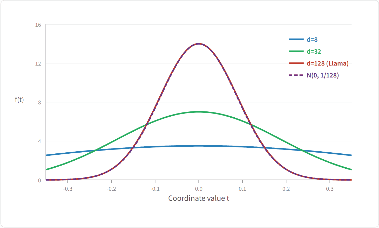
Figure 8. The Beta distribution of coordinates after rotation. At \(d=128\) (Llama's head dimension) it nearly coincides with the Gaussian. Since the distribution is known in advance, the optimal codebook can be designed without any data.

At \(d=128\) the Beta distribution and the Gaussian approximation are nearly indistinguishable. More importantly, in high dimensions different coordinates behave nearly independently. As a result, quantizing each coordinate individually with a scalar quantizer gives almost the same quality as quantizing the whole vector at once with vector quantization.

Sanity check: do the coordinates after rotation follow a Beta distribution?

import numpy as np
from scipy.stats import beta, kstest
d = 128
X = np.random.randn(10000, d)
X /= np.linalg.norm(X, axis=1, keepdims=True)  # normalize onto the unit sphere
coords = X[:, 0]  # take only the first coordinate

# theory: (coord+1)/2 ~ Beta((d-1)/2, (d-1)/2)
a = (d - 1) / 2
_, p_value = kstest((coords + 1) / 2, beta(a, a).cdf)
print(f"KS test p-value: {p_value:.3f}")  # > 0.05 means it matches Beta

# compare quantiles directly too
for q in [0.05, 0.5, 0.95]:
    emp = np.quantile(coords, q)
    theo = 2 * beta(a, a).ppf(q) - 1
    print(f"q={q}: empirical {emp:+.4f}  Beta {theo:+.4f}")

import numpy as np
from scipy.stats import beta, kstest
d = 128
X = np.random.randn(10000, d)
X /= np.linalg.norm(X, axis=1, keepdims=True)  # normalize onto the unit sphere
coords = X[:, 0]  # take only the first coordinate

# theory: (coord+1)/2 ~ Beta((d-1)/2, (d-1)/2)
a = (d - 1) / 2
_, p_value = kstest((coords + 1) / 2, beta(a, a).cdf)
print(f"KS test p-value: {p_value:.3f}")  # > 0.05 means it matches Beta

# compare quantiles directly too
for q in [0.05, 0.5, 0.95]:
    emp = np.quantile(coords, q)
    theo = 2 * beta(a, a).ppf(q) - 1
    print(f"q={q}: empirical {emp:+.4f}  Beta {theo:+.4f}")

import numpy as np
from scipy.stats import beta, kstest
d = 128
X = np.random.randn(10000, d)
X /= np.linalg.norm(X, axis=1, keepdims=True)  # normalize onto the unit sphere
coords = X[:, 0]  # take only the first coordinate

# theory: (coord+1)/2 ~ Beta((d-1)/2, (d-1)/2)
a = (d - 1) / 2
_, p_value = kstest((coords + 1) / 2, beta(a, a).cdf)
print(f"KS test p-value: {p_value:.3f}")  # > 0.05 means it matches Beta

# compare quantiles directly too
for q in [0.05, 0.5, 0.95]:
    emp = np.quantile(coords, q)
    theo = 2 * beta(a, a).ppf(q) - 1
    print(f"q={q}: empirical {emp:+.4f}  Beta {theo:+.4f}")

Designing the Optimal Codebook Without Data

Since the distribution \(f_{X}(t)\) is known analytically, we can solve for the optimal scalar quantizer as a 1D k-means problem:

\[C(f_{X},b):=\min_{-1\le c_{1}\le \cdots \le c_{2^{b}}\le 1}\sum_{i=1}^{2^{b}}\int |x-c_{i}|^{2}\cdot f_{X}(x)dx\]

This is solved by Lloyd-Max. Think of it as 1D k-means; with only one dimension it converges very quickly:

1. Boundary update: given current centroids \(c_{1},\ldots ,c_{2^{b}}\), set the boundary between adjacent regions to the midpoint \((c_{i}+c_{i+1})/2\). (Equivalent to assigning each point to its nearest centroid.)

2. Centroid update: within each region, set the new centroid to the conditional expectation under \(f_{X}\): \(c_{i}\leftarrow \mathbb{E}[X|X\in \text{region}_{i}]\). This is the optimal representative within that region (it minimizes MSE).

3. Repeat 1-2 until convergence.

The crucial point is that, because \(f_{X}\) is known analytically (the Beta distribution above), the integrals can be computed numerically with arbitrary precision. No data samples are required. You converge once, and the resulting codebook is reused forever, across every model, every layer, every token.

Lloyd-Max for a 2-bit codebook

import numpy as np

def lloyd_max_gaussian(n_centroids, sigma=1.0, iters=100):
    """Lloyd-Max for N(0, sigma²), approximated from samples."""
    samples = np.random.randn(100000) * sigma   # approximate the pdf with a large sample
    centroids = np.linspace(-2*sigma, 2*sigma, n_centroids)  # initialization
    for _ in range(iters):
        # Step 1: assign each sample to its nearest centroid
        idx = np.argmin(np.abs(samples[:, None] - centroids), axis=1)
        # Step 2: update each centroid to the mean of its group
        for i in range(n_centroids):
            if np.any(idx == i):
                centroids[i] = samples[idx == i].mean()
    return np.sort(centroids)

# at d=128, coordinates ~ N(0, 1/d), 2-bit (4 centroids)
d = 128
centroids = lloyd_max_gaussian(4, sigma=1/np.sqrt(d))
print(centroids * np.sqrt(d))  # ≈ [-1.51, -0.453, 0.453, 1.51]

import numpy as np

def lloyd_max_gaussian(n_centroids, sigma=1.0, iters=100):
    """Lloyd-Max for N(0, sigma²), approximated from samples."""
    samples = np.random.randn(100000) * sigma   # approximate the pdf with a large sample
    centroids = np.linspace(-2*sigma, 2*sigma, n_centroids)  # initialization
    for _ in range(iters):
        # Step 1: assign each sample to its nearest centroid
        idx = np.argmin(np.abs(samples[:, None] - centroids), axis=1)
        # Step 2: update each centroid to the mean of its group
        for i in range(n_centroids):
            if np.any(idx == i):
                centroids[i] = samples[idx == i].mean()
    return np.sort(centroids)

# at d=128, coordinates ~ N(0, 1/d), 2-bit (4 centroids)
d = 128
centroids = lloyd_max_gaussian(4, sigma=1/np.sqrt(d))
print(centroids * np.sqrt(d))  # ≈ [-1.51, -0.453, 0.453, 1.51]

import numpy as np

def lloyd_max_gaussian(n_centroids, sigma=1.0, iters=100):
    """Lloyd-Max for N(0, sigma²), approximated from samples."""
    samples = np.random.randn(100000) * sigma   # approximate the pdf with a large sample
    centroids = np.linspace(-2*sigma, 2*sigma, n_centroids)  # initialization
    for _ in range(iters):
        # Step 1: assign each sample to its nearest centroid
        idx = np.argmin(np.abs(samples[:, None] - centroids), axis=1)
        # Step 2: update each centroid to the mean of its group
        for i in range(n_centroids):
            if np.any(idx == i):
                centroids[i] = samples[idx == i].mean()
    return np.sort(centroids)

# at d=128, coordinates ~ N(0, 1/d), 2-bit (4 centroids)
d = 128
centroids = lloyd_max_gaussian(4, sigma=1/np.sqrt(d))
print(centroids * np.sqrt(d))  # ≈ [-1.51, -0.453, 0.453, 1.51]

The MSE values in the table above (0.36, 0.117, ...) decay at a rate that's worth understanding in general. The closed-form description is the Panter-Dite high-resolution formula. Derived by Panter and Dite in 1951, it gives an MSE upper bound for a \(b\)-bit optimal scalar quantizer when the distribution \(f_{X}\) is known:

\[C(f_{X},b)\le \frac{1}{12} \bigg( \int f_{X}(x)^{1/3}dx \bigg) ^{3}\cdot \frac{1}{4^{b}}\]

In the TurboQuant context \(f_{X}\) is the post-rotation Beta distribution; computing the integral gives \(C(f_{X},b)\le \frac{\sqrt{3}\pi }{2d}\cdot \frac{1}{4^{b}}\). This formula plays a central role in the distortion bound derivation later. It's tight when \(b\) is large (high-resolution regime); when \(b\) is small the actual values in the table above are even better than the approximation.

The Bias Problem of MSE-Optimal Quantizers

Here's where things get tricky. If you use an MSE-minimizing quantizer to estimate inner products, the result is consistently scaled down by a fixed ratio.

To see why, look at the \(b=1\) case. The 1-bit MSE-optimal codebook is \(\{\pm c\}\) with \(c=\sqrt{2/(\pi d)}\), and the quantized coordinate is \(\hat{x}_{j}=c\cdot \text{sign}(x_{j})\).

To compute the expected inner product, apply the same decomposition as in the QJL proof of section 3: split \(y\) into components parallel and perpendicular to \(x\). The perpendicular component has zero expectation and disappears, leaving only the parallel piece:

\[\mathbb{E}[\langle y,\hat{x}\rangle ]=c\cdot \frac{\langle y,x\rangle }{\|x\|_{2}^{2}}\cdot \mathbb{E} \Bigg[ \sum_{j}|x_{j}| \Bigg] =c\cdot \frac{\langle y,x\rangle }{\|x\|_{2}^{2}}\cdot \mathbb{E}[\|x\|_{1}]\]

(The fact that \(x_{j}\cdot \text{sign}(x_{j})=|x_{j}|\) on the parallel side is the same step 2 from the QJL proof.)

For unit-sphere vectors (\(\|x\|_{2}=1\)), using the approximation \(x_{j}\sim N(0,1/d)\) gives \(\mathbb{E}[|x_{j}|]=\sqrt{2/(\pi d)}\), so:

\[\mathbb{E}[\|x\|_{1}]=d\cdot \sqrt{\frac{2}{\pi d}}=\sqrt{\frac{2d}{\pi }}\]

Substituting:

\[\mathbb{E}[\langle y,\hat{x}\rangle ]=\underbrace{\sqrt{\frac{2}{\pi d}}}_{c}\cdot \langle y,x\rangle \cdot \underbrace{\sqrt{\frac{2d}{\pi }}}_{\mathbb{E}[\|x\|_{1}]}=\sqrt{\frac{2}{\pi d}\cdot \frac{2d}{\pi }}\cdot \langle y,x\rangle =\sqrt{\frac{4}{\pi ^{2}}}\cdot \langle y,x\rangle =\frac{2}{\pi }\langle y,x\rangle\]

That's \(2/\pi \approx 0.637\), or a 36% underestimate. The structure is that the product of \(c\) (the codebook value) and \(\mathbb{E}[\|x\|_{1}]\) (the expected L1 norm) cancels the \(d\), leaving only \(\sqrt{4/\pi ^{2}}=2/\pi\).

The natural question: why not just multiply by \(\pi /2\) to fix it? For \(b=1\), this actually works — \(2/\pi\) is an input-independent constant, so \(\pi /2\cdot (2/\pi )\cdot \langle y,x\rangle =\langle y,x\rangle\) eliminates the bias.

The trouble starts at \(b\ge 2\). Look at the \(b=2\) codebook: \(\{-1.51/\sqrt{d},-0.453/\sqrt{d},+0.453/\sqrt{d},+1.51/\sqrt{d}\}\). Now each coordinate \(x_{j}\) is assigned not just by sign but by magnitude, to one of the closer or farther centroids. For example:

• \(x_{j}=0.03/\sqrt{d}\) → quantized to \(+0.453/\sqrt{d}\) (inflated 15×)

• \(x_{j}=1.2/\sqrt{d}\) → quantized to \(+1.51/\sqrt{d}\) (inflated 26%)

• \(x_{j}=0.9/\sqrt{d}\) → quantized to \(+0.453/\sqrt{d}\) (cut roughly in half)

The quantization error of each coordinate depends on the actual value of \(x_{j}\), in both direction and magnitude. The way these errors contribute to the inner product \(\sum y_{j}\hat{x}_{j}\) also depends on \(y\). As a result, the inner-product bias at \(b=2\) becomes an input-dependent quantity that varies with each pair \((x,y)\), and no single scalar correction works for every input [4].

This is why TurboQuant uses a QJL residual correction instead of simple scaling: QJL is unbiased for whatever residual \(r\) you feed it, so it cleanly removes the bias regardless of \(b\) (1 or 4) or which \((x,y)\) you use. And because QJL is applied to the small residual rather than the full vector, the variance also stays small.

2/π bias at b=1

import numpy as np
d = 128; trials = 5000
c1 = np.sqrt(2 / (np.pi * d))  # b=1 codebook

# Setting y = x makes <y, x> = 1 and <y, x_q> = c·||x||_1, so we land on exactly 2/π
ratios = []
for _ in range(trials):
    x = np.random.randn(d); x /= np.linalg.norm(x)
    x_q = c1 * np.sign(x)               # 1-bit MSE quantization
    ratios.append(x @ x_q)               # <x, x_q> = c·||x||_1

print(f"<x, x_q> mean: {np.mean(ratios):.4f}")  # ≈ 0.6366
print(f"theoretical 2/π: {2/np.pi:.4f}")         # 0.6366
# → at b=1 the bias is a constant, so π/2 corrects it. But at b≥2
#   the codebook is more complex, the bias becomes input-dependent,
#   and no single scalar correction works.

import numpy as np
d = 128; trials = 5000
c1 = np.sqrt(2 / (np.pi * d))  # b=1 codebook

# Setting y = x makes <y, x> = 1 and <y, x_q> = c·||x||_1, so we land on exactly 2/π
ratios = []
for _ in range(trials):
    x = np.random.randn(d); x /= np.linalg.norm(x)
    x_q = c1 * np.sign(x)               # 1-bit MSE quantization
    ratios.append(x @ x_q)               # <x, x_q> = c·||x||_1

print(f"<x, x_q> mean: {np.mean(ratios):.4f}")  # ≈ 0.6366
print(f"theoretical 2/π: {2/np.pi:.4f}")         # 0.6366
# → at b=1 the bias is a constant, so π/2 corrects it. But at b≥2
#   the codebook is more complex, the bias becomes input-dependent,
#   and no single scalar correction works.

import numpy as np
d = 128; trials = 5000
c1 = np.sqrt(2 / (np.pi * d))  # b=1 codebook

# Setting y = x makes <y, x> = 1 and <y, x_q> = c·||x||_1, so we land on exactly 2/π
ratios = []
for _ in range(trials):
    x = np.random.randn(d); x /= np.linalg.norm(x)
    x_q = c1 * np.sign(x)               # 1-bit MSE quantization
    ratios.append(x @ x_q)               # <x, x_q> = c·||x||_1

print(f"<x, x_q> mean: {np.mean(ratios):.4f}")  # ≈ 0.6366
print(f"theoretical 2/π: {2/np.pi:.4f}")         # 0.6366
# → at b=1 the bias is a constant, so π/2 corrects it. But at b≥2
#   the codebook is more complex, the bias becomes input-dependent,
#   and no single scalar correction works.

Two-Stage Approach: MSE Approximation + QJL Correction

TurboQuant's solution is to split the \(b\)-bit budget into two stages: \((b-1)\) bits for MSE quantization (a coarse approximation), the remaining 1 bit for QJL residual correction (a precise fix).

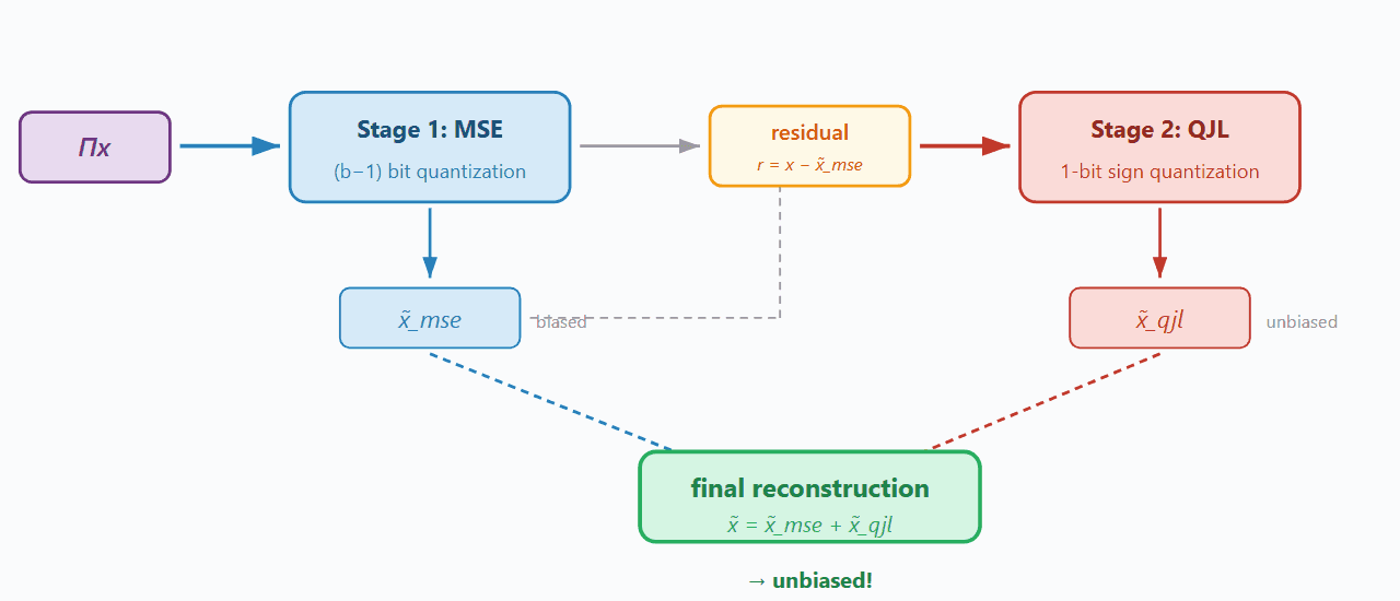
Figure 9. TurboQuant's two-stage pipeline. Stage 1 (MSE) provides a coarse approximation; Stage 2 (QJL) corrects the residual without bias.

In equations:

Stage 1 — MSE quantization (\(b-1\) bits):

\[\hat{x}_{\text{mse}}=\text{DeQuant}_{\text{mse}}(\text{Quant}_{\text{mse}}(x)),r=x-\hat{x}_{\text{mse}}\]

Stage 2 — QJL residual correction (1 bit):

\[\hat{x}_{\text{qjl}}=\frac{\sqrt{\pi /2}}{d}\|r\|_{2}S^{\top }\cdot \text{sign}(S\cdot r)\]

Final reconstruction: \(\hat{x}=\hat{x}_{\text{mse}}+\hat{x}_{\text{qjl}}\)

TurboQuant two-stage pipeline

import numpy as np
d = 128; trials = 2000
codebook = np.array([-1.51, -0.453, 0.453, 1.51]) / np.sqrt(d)  # 2-bit

mse_only, with_qjl, truth = [], [], []
for _ in range(trials):
    x = np.random.randn(d); x /= np.linalg.norm(x)
    y = np.random.randn(d); y /= np.linalg.norm(y)
    Pi = np.linalg.qr(np.random.randn(d, d))[0]  # random orthogonal

    # Stage 1: 2-bit MSE quantization after rotation
    rot = Pi @ x
    idx = np.argmin(np.abs(rot[:, None] - codebook), axis=1)
    x_mse = Pi.T @ codebook[idx]

    # Stage 2: 1-bit QJL on the residual
    r = x - x_mse
    S = np.random.randn(d, d)
    x_qjl = np.sqrt(np.pi/2) / d * np.linalg.norm(r) * S.T @ np.sign(S @ r)

    truth.append(y @ x)
    mse_only.append(y @ x_mse)
    with_qjl.append(y @ (x_mse + x_qjl))

# Measure bias via regression slope (1.0 means unbiased)
slope = lambda est: np.dot(est, truth) / np.dot(truth, truth)
print(f"MSE only slope:    {slope(mse_only):.4f}")   # < 1 (biased)
print(f"MSE + QJL slope:   {slope(with_qjl):.4f}")  # ≈ 1 (unbiased!)

import numpy as np
d = 128; trials = 2000
codebook = np.array([-1.51, -0.453, 0.453, 1.51]) / np.sqrt(d)  # 2-bit

mse_only, with_qjl, truth = [], [], []
for _ in range(trials):
    x = np.random.randn(d); x /= np.linalg.norm(x)
    y = np.random.randn(d); y /= np.linalg.norm(y)
    Pi = np.linalg.qr(np.random.randn(d, d))[0]  # random orthogonal

    # Stage 1: 2-bit MSE quantization after rotation
    rot = Pi @ x
    idx = np.argmin(np.abs(rot[:, None] - codebook), axis=1)
    x_mse = Pi.T @ codebook[idx]

    # Stage 2: 1-bit QJL on the residual
    r = x - x_mse
    S = np.random.randn(d, d)
    x_qjl = np.sqrt(np.pi/2) / d * np.linalg.norm(r) * S.T @ np.sign(S @ r)

    truth.append(y @ x)
    mse_only.append(y @ x_mse)
    with_qjl.append(y @ (x_mse + x_qjl))

# Measure bias via regression slope (1.0 means unbiased)
slope = lambda est: np.dot(est, truth) / np.dot(truth, truth)
print(f"MSE only slope:    {slope(mse_only):.4f}")   # < 1 (biased)
print(f"MSE + QJL slope:   {slope(with_qjl):.4f}")  # ≈ 1 (unbiased!)

import numpy as np
d = 128; trials = 2000
codebook = np.array([-1.51, -0.453, 0.453, 1.51]) / np.sqrt(d)  # 2-bit

mse_only, with_qjl, truth = [], [], []
for _ in range(trials):
    x = np.random.randn(d); x /= np.linalg.norm(x)
    y = np.random.randn(d); y /= np.linalg.norm(y)
    Pi = np.linalg.qr(np.random.randn(d, d))[0]  # random orthogonal

    # Stage 1: 2-bit MSE quantization after rotation
    rot = Pi @ x
    idx = np.argmin(np.abs(rot[:, None] - codebook), axis=1)
    x_mse = Pi.T @ codebook[idx]

    # Stage 2: 1-bit QJL on the residual
    r = x - x_mse
    S = np.random.randn(d, d)
    x_qjl = np.sqrt(np.pi/2) / d * np.linalg.norm(r) * S.T @ np.sign(S @ r)

    truth.append(y @ x)
    mse_only.append(y @ x_mse)
    with_qjl.append(y @ (x_mse + x_qjl))

# Measure bias via regression slope (1.0 means unbiased)
slope = lambda est: np.dot(est, truth) / np.dot(truth, truth)
print(f"MSE only slope:    {slope(mse_only):.4f}")   # < 1 (biased)
print(f"MSE + QJL slope:   {slope(with_qjl):.4f}")  # ≈ 1 (unbiased!)

One thing worth noting: in section 3 we said QJL could only estimate inner products, but here \(\frac{\sqrt{\pi /2}}{d}\|r\|S^{\top }\cdot \text{sign}(S\cdot r)\) is "reconstructing" the vector itself. \(S^{\top }\) here is not the inverse of \(S\) — \(S\) is a Gaussian random matrix, not an orthogonal one, so \(S^{\top }S\not =I\). What \(S^{\top }\) does here is not a linear-algebraic inverse but a back-projection estimator that maps the sign information from random projections back to the original space. This estimator is unbiased for the same reason from section 3 (the half-normal property of Gaussian projections), and setting \(m=d\) gives \(d\) independent votes, which keeps the variance small. Thanks to this, TurboQuant\(_{\text{prod}}\) can also be applied to the value cache.

How is this different from PolarQuant's reconstruction?

Both methods can "reconstruct vectors," but they work on completely different principles:

• PolarQuant: the polar transform is deterministic and exactly invertible. Without quantization, \((x_{1},x_{2})\to (r,\psi )\to (r\cos \psi ,r\sin \psi )\) recovers the original perfectly. Quantization error only enters through the discretization of the angles. This relies on the geometric invertibility of a coordinate change.

• TurboQuant's \(S^{\top }\) step: not deterministically invertible. Applying \(S^{\top }\) doesn't bring back the original exactly — it only matches on average, in the sense that \(\mathbb{E}[\hat{r}]=r\). There's noise on every individual estimate, and the variance is reduced by averaging over \(d\) rows. This is a statistical estimator.

An analogy: PolarQuant is like "Korean → English → Korean translation" (a 1:1 correspondence), while TurboQuant's QJL stage is like "asking 100 people for a rating and averaging" (each individual is noisy, but the average converges to the truth). Both end up with the same outcome (applicability to the value cache), but TurboQuant didn't borrow PolarQuant's reconstruction approach — it gets the same capability through a completely different mechanism (statistical averaging).

This difference creates a meaningful trade-off in practice.

As the table shows, the two methods win on different axes:

• TurboQuant's strengths (speed and theory): the dequant path is just matmul + lookup, which is overwhelmingly faster on GPU/NPU. In particular, the trick \(\langle q,\tilde{x}\rangle =\langle \Pi q,\tilde{y}\rangle\) lets you compute \(\Pi q\) just once per query, after which each cached token only needs an \(O(d)\) inner product. PolarQuant has to call \(d\) cos/sin's recursively for every token. There's also the clean theoretical guarantee of being within ~2.7× of the Shannon lower bound.

• PolarQuant's strengths (stability): deterministic reconstruction and softmax-friendliness. It can be more robust at small head_dim or in tricky attention layers.

For most realistic scenarios (large-scale LLM serving, GPU inference) speed and hardware friendliness are decisive, so TurboQuant has the edge. That's why Google promotes it as the main approach, and why most recent community implementations (llama.cpp, vLLM) are TurboQuant variants. That said, as we'll see in section 7, TurboQuant's QJL stage has the softmax-variance-amplification trap, so in practice many implementations use only the MSE stage. In that case "TurboQuant\(_{\text{mse}}\)" approaches PolarQuant's deterministic stability while keeping the speed advantage.

Unbiasedness Proof

I personally find this proof to be the cleanest part of the paper. QJL is unbiased for any input vector, so it's also unbiased on the residual \(r\). Applying total expectation:

\[\mathbb{E}[\langle y,\hat{x}\rangle ]=\underbrace{\mathbb{E}[\langle y,\hat{x}_{\text{mse}}\rangle ]}_{\text{biased}}+\underbrace{\langle y,x\rangle -\mathbb{E}[\langle y,\hat{x}_{\text{mse}}\rangle ]}_{\text{QJL estimates the residual unbiasedly}}=\langle y,x\rangle\]

The \(\mathbb{E}[\langle y,\hat{x}_{\text{mse}}\rangle ]\) terms cancel exactly between the \(+\) and \(-\) sides. Whatever bias the MSE stage has, QJL automatically compensates for it by estimating the residual without bias. And since Stage 1 shrinks the residual, Stage 2's variance also shrinks — a rather elegant synergy.

Variance Bound and 1/4^b Scaling

Now that we have unbiasedness, the remaining question is how small the error is. Here we need to distinguish two error measures:

• \(D_{\text{mse}}\): MSE distortion = \(\mathbb{E}[\|x-\hat{x}\|_{2}^{2}]\). The expected squared Euclidean distance between the original and reconstructed vectors.

• \(D_{\text{prod}}\): inner-product distortion = \(\mathbb{E}[|\langle y,x\rangle -\langle y,\hat{x}\rangle |^{2}]\). The expected squared error of the inner-product estimate for a particular query \(y\). This is directly related to the quality of attention scores.

TurboQuant\(_{\text{mse}}\) minimizes \(D_{\text{mse}}\), while TurboQuant\(_{\text{prod}}\) minimizes \(D_{\text{prod}}\). Below we derive the upper bound on \(D_{\text{prod}}\).

First, the structure of the variance. In the reconstructed vector \(\hat{x}=\hat{x}_{\text{mse}}+\hat{x}_{\text{qjl}}\), the term \(\hat{x}_{\text{mse}}\) is deterministic once the rotation matrix \(\Pi\) is fixed — it always returns the same codebook indices for the same input. The randomness comes only from the matrix \(S\) in the QJL stage. So by the law of total variance:

\[\text{Var}(\langle y,\hat{x}\rangle )=\mathbb{E}_{\hat{x}_{\text{mse}}} \big[ \text{Var}(\langle y,\hat{x}_{\text{qjl}}\rangle |\hat{x}_{\text{mse}}) \big]\]

(Conditioning on \(\hat{x}_{\text{mse}}\) makes \(\langle y,\hat{x}_{\text{mse}}\rangle\) a constant, so \(\text{Var}(\langle y,\hat{x}_{\text{mse}}\rangle |\hat{x}_{\text{mse}})=0\).)

Now we bound the conditional variance. Given \(\hat{x}_{\text{mse}}\), the residual \(r=x-\hat{x}_{\text{mse}}\) is a fixed vector and QJL is applied to it. Recall the QJL dequantization:

\[\hat{x}_{\text{qjl}}=\frac{\sqrt{\pi /2}}{d}\|r\|_{2}S^{\top }\cdot \text{sign}(S\cdot r)\]

We need the variance of \(\langle y,\hat{x}_{\text{qjl}}\rangle\). For each row \(s_{i}\) of \(S\), the \(i\)-th "vote" of the estimator is \(\sqrt{\pi /2}\|r\|_{2}(s_{i}^{\top }y)\text{sign}(s_{i}^{\top }r)\). To bound its variance, we just compute the second moment (since Var \(\le\) E[X²]).

Because \(\text{sign}(s_{i}^{\top }r)\in \{-1,+1\}\), squaring it always gives 1:

\[\big[ (s_{i}^{\top }y)\text{sign}(s_{i}^{\top }r) \big] ^{2}=(s_{i}^{\top }y)^{2}\cdot \underbrace{\text{sign}(s_{i}^{\top }r)^{2}}_{=1}=(s_{i}^{\top }y)^{2}\]

So the sign function disappears cleanly and the second moment reduces to the expectation of \((s_{i}^{\top }y)^{2}\). Since \(s_{i}\) is Gaussian, \(s_{i}^{\top }y\sim N(0,\|y\|^{2})\) and:

\[\mathbb{E}[(s_{i}^{\top }y)^{2}]=\|y\|_{2}^{2}\]

Including the correction factor \(\sqrt{\pi /2}\) and \(\|r\|\):

\[\text{Var} \big( \sqrt{\pi /2}\|r\|_{2}(s_{i}^{\top }y)\text{sign}(s_{i}^{\top }r) \big) \le \frac{\pi }{2}\|r\|_{2}^{2}\|y\|_{2}^{2}\]

Averaging over \(d\) rows (independent, so the variance shrinks by \(1/d\)):

\[\text{Var}(\langle y,\hat{x}_{\text{qjl}}\rangle |\hat{x}_{\text{mse}})\le \frac{1}{d}\cdot \frac{\pi }{2}\|y\|_{2}^{2}\|r\|_{2}^{2}=\frac{\pi }{2d}\|y\|_{2}^{2}\cdot \|r\|_{2}^{2}\]

That's where \(\pi /(2d)\) comes from: \(\pi /2\) is the squared QJL correction factor (\((\sqrt{\pi /2})^{2}\)), and \(1/d\) is from averaging \(d\) independent votes. The structure is that the smaller Stage 1 makes \(r\), the smaller this variance becomes.

Taking the expectation over \(\hat{x}_{\text{mse}}\):

\[D_{\text{prod}}(b)\le \frac{\pi }{2d}\|y\|_{2}^{2}\cdot \underbrace{\mathbb{E}[\|r\|_{2}^{2}]}_{\text{Stage 1’s total MSE}}\]

Now compute \(\mathbb{E}[\|r\|_{2}^{2}]\). This is the total reconstruction error of \((b-1)\)-bit MSE quantization, i.e. the sum of the per-coordinate quantization errors over all \(d\) coordinates:

\[\mathbb{E}[\|r\|_{2}^{2}]=\sum_{j=1}^{d}\mathbb{E}[(x_{j}-\hat{x}_{j})^{2}]=d\cdot C(f_{X},b-1)\]

where \(C(f_{X},b-1)\) is the per-coordinate MSE of a single coordinate. By the Panter-Dite high-resolution formula [4]:

\[C(f_{X},b-1)\le \frac{\sqrt{3}\pi }{2d}\cdot \frac{1}{4^{b-1}}\]

Putting it all together:

\[D_{\text{prod}}(b)\le \frac{\pi }{2d}\|y\|_{2}^{2}\cdot d\cdot \frac{\sqrt{3}\pi }{2d}\cdot \frac{1}{4^{b-1}}\]

Simplifying (\(d\) cancels and \(1/4^{b-1}=4/4^{b}\)):

\[=\frac{\pi }{2d}\cdot d\cdot \frac{\sqrt{3}\pi }{2d}\cdot \frac{4}{4^{b}}\cdot \|y\|_{2}^{2}=\frac{4\sqrt{3}\pi ^{2}}{4d}\cdot \frac{\|y\|_{2}^{2}}{4^{b}}=\frac{\sqrt{3}\pi ^{2}}{d}\|y\|_{2}^{2}\cdot \frac{1}{4^{b}}\]

The mechanism: Stage 1 achieves an MSE of \(1/4^{b-1}\) with \(b-1\) bits, and Stage 2's QJL multiplies by a \(\pi /(2d)\cdot d=\pi /2\) factor while introducing an additional \(4\) in the denominator, ending at \(1/4^{b}\). Each additional bit reduces the error by a factor of 4.

Comparison with Information-Theoretic Lower Bounds

We've derived the upper bound; now let's see the lower bound that says "you can't do better than this with any method."

The lower-bound argument has two steps [4]:

Step 1 — Yao's minimax principle. What we want is "the optimal (random) quantization algorithm's error on the worst-case input." In equations:

\[\min_{\text{random algorithm }Q}\max_{\text{input }x}\mathbb{E}[\text{error}(Q,x)]\]

This is hard to attack directly — we have to handle "worst-case input" and "optimal random algorithm" at the same time. Yao's minimax principle flips it around:

\[\min_{\text{random }Q}\max_{x}\mathbb{E}[\text{error}]=\max_{\text{input distribution }P}\min_{\text{deterministic }Q}\mathbb{E}_{x\sim P}[\text{error}]\]

The left side (the original problem) is the worst case of a random algorithm; the right side (the transformed problem) is the average case of a deterministic algorithm. The transformed version is much easier to handle: choosing the uniform distribution on the unit sphere \(S^{d-1}\) as the "worst distribution" \(P\) lets us apply Shannon's rate-distortion theory directly.

Step 2 — Shannon's lossy source coding theorem. Now the input comes from the uniform distribution on \(S^{d-1}\). By Shannon's rate-distortion theory, the lower bound on the achievable MSE when encoding a \(d\)-dimensional vector with a total of \(B=b\cdot d\) bits is:

\[D_{\text{mse}}\ge 2^{-2B/d}=2^{-2b}=\frac{1}{4^{b}}\]

For the lower bound on \(D_{\text{prod}}\) we go one more step using the pigeonhole principle. Decompose the total MSE coordinate-wise:

\[D_{\text{mse}}=\sum_{j=1}^{d}\mathbb{E}[|x_{j}-\hat{x}_{j}|^{2}]\ge \frac{1}{4^{b}}\]

Since the sum of \(d\) terms is at least \(1/4^{b}\), there exists at least one coordinate \(j^{*}\) such that:

\[\mathbb{E}[|x_{j^{*}}-\hat{x}_{j^{*}}|^{2}]\ge \frac{1}{d\cdot 4^{b}}\]

Choosing \(y=e_{j^{*}}\) (the standard basis vector with \(\|e_{j^{*}}\|=1\)), we get \(\langle e_{j^{*}},x-\hat{x}\rangle =x_{j^{*}}-\hat{x}_{j^{*}}\), so:

\[D_{\text{prod}}=\mathbb{E}[|\langle e_{j^{*}},x-\hat{x}\rangle |^{2}]\ge \frac{1}{d\cdot 4^{b}}\]

This is the special case where \(\|y\|=1\); for general \(y\), \(D_{\text{prod}}\) is proportional to \(\|y\|^{2}\), so:

\[D_{\text{prod}}(Q)\ge \frac{\|y\|^{2}}{d}\cdot \frac{1}{4^{b}}\]

To summarize, the two lower bounds are:

\[D_{\text{mse}}(Q)\ge \frac{1}{4^{b}},D_{\text{prod}}(Q)\ge \frac{\|y\|^{2}}{d}\cdot \frac{1}{4^{b}}\]

Upper vs. lower bound:

For MSE distortion, TurboQuant's upper bound is \(\frac{\sqrt{3}\pi }{2}\cdot \frac{1}{4^{b}}\) and the lower bound is \(\frac{1}{4^{b}}\), so the ratio is \(\sqrt{3}\pi /2\approx 2.72\) — i.e. within roughly 2.7× of the information-theoretic optimum. At \(b=1\) the gap shrinks further to about 1.45×.

For inner-product distortion, the asymptotic ratio of upper to lower bound is \(\sqrt{3}\pi ^{2}\approx 17.1\), larger than for MSE. But this number comes from the Panter-Dite high-resolution approximation, and the actual gap at low bit widths is much smaller.

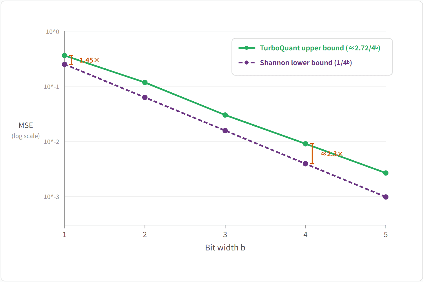
Figure 10. Comparison of MSE distortion rates. TurboQuant scales as \(1/4^{b}\), staying within roughly 2.7× of the Shannon lower bound.

That said, the structure "normalize → random rotation → coordinate quantization → unbiased estimation" wasn't introduced by TurboQuant. There's something we should address before moving on.

The RaBitQ Connection (and Controversy)

RaBitQ (Gao & Long, SIGMOD 2024) [5] shares a similar structure with TurboQuant — normalize → random orthogonal rotation → coordinate quantization → unbiased estimator. However, RaBitQ always quantizes to one bit per coordinate (vertices of the hypercube \(\{-1/\sqrt{D},+1/\sqrt{D}\}^{D}\)), and to support multiple bits it has to expand the dimension via zero-padding. TurboQuant uses Lloyd-Max codebooks optimized for the Beta distribution at any \(b\). Both reduce to taking the sign at \(b=1\), but the codebook values differ (TurboQuant: \(\pm \sqrt{2/\pi d}\), RaBitQ: \(\pm 1/\sqrt{D}\)) and so do the inner-product estimators (TurboQuant uses QJL, while RaBitQ uses a ratio estimator \(\langle \bar{o},q\rangle /\langle \bar{o},o\rangle\)). The proof of optimality relative to the Shannon lower bound and support for arbitrary bit widths are TurboQuant's distinct contributions.

That said, the relationship between the two methods is currently under dispute. The RaBitQ authors have publicly raised concerns that TurboQuant did not adequately describe its structural similarity to RaBitQ (in particular regarding JL/random rotation), that the theoretical comparison is inaccurate, and that the experimental conditions are insufficiently disclosed [26]. The discussion was also addressed in the ICLR 2026 review process and is preserved as a public record at the community level.

Practical Issues Found in Implementation

From late 2025 onward, llama.cpp, vLLM, and independent researchers started implementing the TurboQuant family, and in the process several issues that the paper didn't anticipate came to light.

QJL Residual Correction's Practical Limitations

When I first read the paper, I thought the QJL residual correction was the cleanest part — but practical results turned out the opposite.

Multiple independent implementation teams [9][10] arrived at the same conclusion: applying the QJL residual correction often hurts quality. A llama.cpp community discussion [14] reported that, on a GPT-2 with head_dim=64, applying QJL increased perplexity by 300%; in scos-lab's reproduction [16], MSE-only (+1.1% PPL) significantly outperformed MSE+QJL (+6.5% PPL).

This conclusion isn't universal, however. 0xSero/turboquant [11] includes QJL as a core stage of its pipeline and reports a cosine similarity of 1.000000 on 3-bit keys, and hackimov/turboquant-kv [32] also uses QJL by default. sharpner/turboquant-mlx [33] offers QJL as an optional setting and reports a small quality improvement at 3-bit (+6.6% → +5.3%) at the cost of about a 30% slowdown.

The cause is variance amplification through softmax. The QJL estimator is unbiased for inner products, but its variance is not zero. Attention scores feed inner products through softmax, and softmax is nonlinear, so:

\[\mathbb{E}[\text{softmax}(\hat{s}_{1},\ldots ,\hat{s}_{n})]\not =\text{softmax}(\mathbb{E}[\hat{s}_{1}],\ldots ,\mathbb{E}[\hat{s}_{n}])\]

In other words, even if the inner products are unbiased, the softmax outputs are not. The variance the QJL stage adds gets amplified through softmax. As a result, in practice TurboQuant\(_{\text{mse}}\) — the version that uses only the MSE stage and skips the QJL residual correction — often performs better. To put it another way: TurboQuant's Theorem 2 [4] proves unbiasedness for inner-product estimation, not for the softmax-weighted attention output. A low-variance biased estimator (MSE-only) can be more stable after softmax than a high-variance unbiased one (MSE+QJL), and that's the consensus from multiple independent implementations [9][10][14].

Other Practical Constraints

• Theoretical guarantees weaken at small head dimensions: TurboQuant's theory relies on high-dimensional concentration of measure [4], so the approximation works better when \(d\) is large. At \(d=128\) and above the Beta-to-Gaussian convergence is more than sufficient, but at \(d=64\) (used in some models) the codebook optimality guarantee weakens, and the llama.cpp community [14] has reported actual quality degradation.

• K/V asymmetry: confirmed by multiple implementations [10][16] — the value cache can be aggressively compressed to 2 bits with little quality loss, but the key cache is much more sensitive. Models with K/V norm ratios as high as 1274× have been reported [16]. In practice, an asymmetric strategy that gives 4 bits to K and 2 bits to V works well [10].

• Boundary layer sensitivity: keeping the first and last two layers at higher precision recovers 37-91% of the quality loss [10]. This is a practical strategy that diverges from TurboQuant's theoretical assumption of "uniform application across all layers."

• Lack of fused kernels: when dequantization and the attention computation run as separate kernels, intermediate results have to be written out to HBM and read back, wiping out the bandwidth advantage. An early draft PR for vLLM [15] reported that, without a fused kernel, on a particular setup (Qwen2.5-7B, H100) decode throughput dropped to 0.36× the baseline. This will improve as implementations mature, but it shows that integration with FlashAttention is the key to making this practical.

Open-Source Implementation Status

An official Google implementation has not yet been released (as of April 2026) [8], but community implementations are active:

The practical consensus from multiple implementations: the QJL residual correction requires care because of softmax variance amplification. In most cases MSE quantization alone is enough [9][10][14][16], and asymmetric K/V bit allocation plus boundary-layer protection is effective. That said, some implementations [11] report positive results from QJL, so validation per model and per hardware is recommended.

Running TurboQuant on NPUs

TurboQuant's core operations are three: (1) Hadamard transform (energy spreading), (2) codebook lookup (quantization/dequantization), (3) low-bit integer packing/unpacking. How well these three map to current NPU hardware is what determines whether TurboQuant becomes practical.

The Hadamard transform is, surprisingly, not natively supported on most NPUs. On NVIDIA Tensor Cores, the HadaCore technique can map it to 16x16 mma instructions, but that's a software optimization that exploits the Hadamard structure, not native hardware support. That said, at \(d=128\) the WHT amounts to 7 stages × 64 butterflies = roughly 900 add/subs, so even without native support it can be processed quickly enough on the vector unit. The actual bottleneck for TurboQuant isn't Hadamard — it's memory bandwidth. Still, future NPU designs that integrate butterfly operations into the datapath could further reduce the preprocessing overhead.

Codebook lookup is one of the NPU's weak points. NPUs are optimized for dense GEMM, so element-wise dequantization can actually be slower than on a CPU. According to T-MAN [31], element-wise float operations on a Qualcomm NPU were 3.8× slower than on the CPU; fusing them into a two-stage LUT yielded a 10.2× speedup. TurboQuant's codebooks are tiny (2-16 entries), which fits a hardware LUT well. Qualcomm Hexagon's VLUT16 instruction is one example of what could be exploited here.

Low-bit support varies widely across hardware:

* Apple ANE supports weight palettization (1-8 bit LUT storage compression) via Core ML, but this is weight-only storage compression and does not directly apply to activation/KV-cache quantization. Also, after dequantization the computation runs in FP16, so the compute is not low-bit.

As the table shows, no NPU yet natively supports 3-bit integers — TurboQuant's main bit width. NVIDIA Blackwell is an interesting case: it dropped the INT4 tensor cores that Hopper had in favor of NVFP4 (a floating-point format) — because floating-point 4-bit handles outliers better, but for codebook quantization like TurboQuant integer indices are still more natural. Native Hadamard support, 3-bit integer arithmetic, and integration of small codebook LUTs into the datapath are the key challenges for future NPU designs.

Pulling the practical lessons together, the heart of the theory — using a random rotation to make the distribution predictable — still holds. QJL's unbiasedness is exact at the inner-product level, but in the nonlinear context of softmax attention, variance management may be more important. The MSE stage that applies the optimal codebook after rotation is where the practical value lives, and the usefulness of QJL depends on the implementation context. On the hardware side, NPU designs matched to TurboQuant's compute profile (Hadamard + low-bit codebook) are starting to emerge.

Wrap-up: Random Rotation as the Core Tool

Running through JL theory (1984/2021) → QJL (2024) → PolarQuant (2025) → TurboQuant (2025), there's one shared principle:

A principle that runs through 40 years

Multiplying by a random orthogonal matrix turns an arbitrary worst-case vector into a random variable with a known distribution.

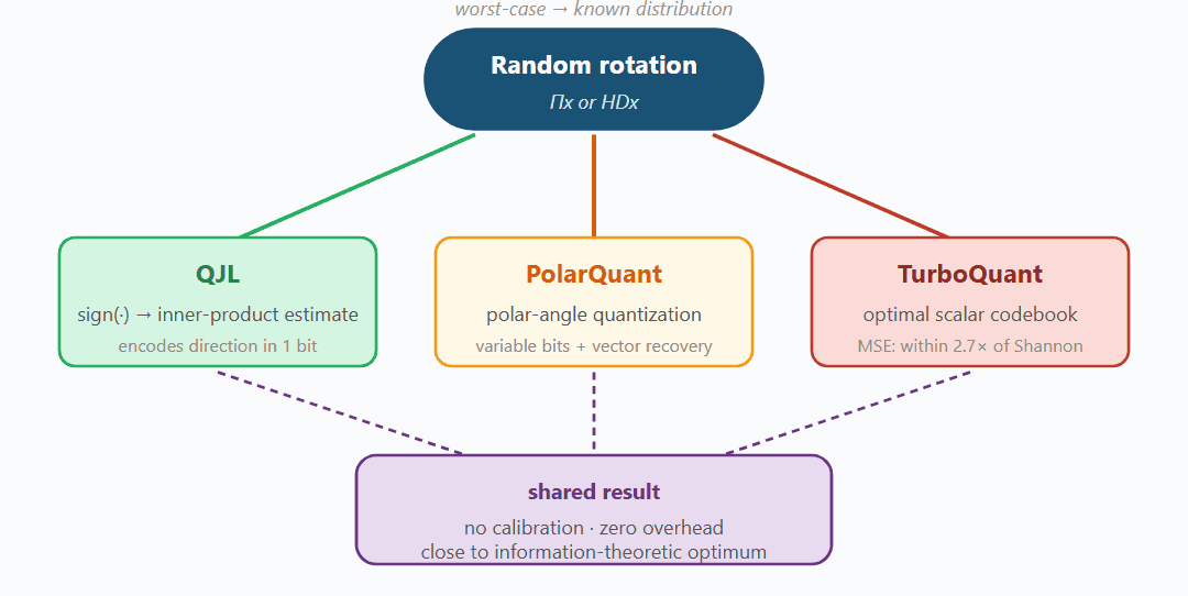
Figure 11. The structure that runs through all four papers. "A single random rotation" is where everything begins.

QJL estimates inner products from sign bits alone, PolarQuant makes the distribution of polar angles predictable, and TurboQuant designs the optimal scalar codebook from the Beta distribution of the coordinates. In all three cases, rotation removes the data dependence.

Of course, there's a gap between theory and practice. QJL's unbiasedness can actually hurt once you go through softmax, because of variance amplification, and the theoretical guarantees weaken at small head dimensions or in boundary layers. There's also an ongoing academic dispute about the structural similarity to RaBitQ. Even so, the core idea — use a random rotation to make the distribution predictable, then design a quantizer matched to that distribution — has survived in practice. The MSE-only quantization the community has adopted (TurboQuant\(_{\text{mse}}\)) is exactly that idea in action.

An idea that started as pure mathematics in 1984 has, after 40 years of evolution, given a theoretical answer to the central bottleneck of LLM inference. The process of refining theory through contact with practice is still very much underway.

References

1. Freksen, C.B. (2021). An Introduction to Johnson-Lindenstrauss Transforms. arXiv:2103.00564

2. Zandieh, A., Daliri, M., Han, I. (2024). QJL: 1-Bit Quantized JL Transform for KV Cache Quantization with Zero Overhead. AAAI 2025. arXiv:2406.03482

3. Han, I., Kacham, P., Karbasi, A., Mirrokni, V., Zandieh, A. (2025). PolarQuant: Quantizing KV Caches with Polar Transformation. AISTATS 2026. arXiv:2502.02617

4. Zandieh, A., Daliri, M., Hadian, M., Mirrokni, V. (2025). TurboQuant: Online Vector Quantization with Near-optimal Distortion Rate. ICLR 2026. arXiv:2504.19874

5. Gao, J., Long, C. (2024). RaBitQ: Quantizing High-Dimensional Vectors with a Theoretical Error Bound for Approximate Nearest Neighbor Search. SIGMOD 2024. arXiv:2405.12497

6. Xiao, G., et al. (2023). SmoothQuant: Accurate and Efficient Post-Training Quantization for Large Language Models. ICML 2023.

7. Liu, Z., et al. (2024). SpinQuant: LLM Quantization with Learned Rotations. ICLR 2025. arXiv:2405.16406

8. Google Research Blog (2026). TurboQuant: Redefining AI Efficiency with Extreme Compression.

9. tonbistudio (2026). turboquant-pytorch: PyTorch TurboQuant implementation. Switched to MSE-only after removing the QJL residual correction.

10. TheTom (2026). turboquant_plus: TurboQuant integration in llama.cpp. turbo2/3/4 formats; validated on Apple/NVIDIA/AMD.

11. 0xSero (2026). turboquant (vLLM): TurboQuant integration in vLLM. Triton kernels, RTX 5090 benchmarks.

12. Gerganov, G. (2026). llama.cpp PR #21038: rotate activations for better quantization: Hadamard rotation to improve KV-cache quantization quality.

13. elusznik (2026). llama.cpp PR #21089: TBQ3_0/TBQ4_0 KV cache quantization: CPU-only TurboQuant formats.

14. llama.cpp community (2026). Discussion #20969: TurboQuant extreme KV cache quantization.

15. vLLM community (2026). vLLM PR #38280: TurboQuant KV cache compression: Draft stage; reports a 0.36× decode drop without fused kernels.

16. scos-lab (2026). turboquant (research reproduction): MSE-based outperforms product-space; reports a K/V norm ratio of 1274×.

17. Ailon, N., Chazelle, B. (2009). The Fast Johnson-Lindenstrauss Transform and Approximate Nearest Neighbors. SIAM J. Comput. 39(1), 302–322.

18. Chee, J., et al. (2024). QuIP: 2-Bit Quantization of Large Language Models With Guarantees. NeurIPS 2023. arXiv:2307.13304

19. Tseng, A., et al. (2024). QuIP#: Even Better LLM Quantization with Hadamard Incoherence and Lattice Codebooks. ICML 2024. arXiv:2402.04396

20. Johnson, W.B., Lindenstrauss, J. (1984). Extensions of Lipschitz mappings into a Hilbert space. Contemporary Mathematics, 26, 189–206.

21. Dasgupta, S., Gupta, A. (2003). An elementary proof of a theorem of Johnson and Lindenstrauss. Random Structures & Algorithms, 22(1), 60–65.

22. Achlioptas, D. (2003). Database-friendly random projections: Johnson-Lindenstrauss with binary coins. J. Comput. Syst. Sci., 66(4), 671–687.

23. Liu, Z., et al. (2024). KIVI: A Tuning-Free Asymmetric 2bit Quantization for KV Cache. ICML 2024. arXiv:2402.02750

24. Hooper, C., et al. (2024). KVQuant: Towards 10 Million Context Length LLM Inference with KV Cache Quantization. NeurIPS 2024. arXiv:2401.18079

25. Vaswani, A., et al. (2017). Attention Is All You Need. NeurIPS 2017. arXiv:1706.03762

26. Long, C. (2026). Concerns from the RaBitQ Authors Regarding Method Description, Theoretical Comparison, and Experimental Disclosure. OpenReview public comment on TurboQuant, March 27, 2026.

27. NVIDIA (2025). NVIDIA Blackwell Architecture. NVFP4/FP8/INT8 support, Transformer Engine.

28. Google (2025). Introducing Trillium, our 6th-generation TPU. TPU v6e (Trillium) / Ironwood specifications.

29. Qualcomm (2024). Qualcomm AI Engine Direct (QNN) SDK Documentation. Hexagon NPU, INT4/INT8 support.

30. Apple (2024). Core ML Tools: Post-Training Palettization. ANE weight palettization (1–8 bit LUT).

31. Park, G., et al. (2025). T-MAN: Enabling End-to-End Low-Bit LLM Inference on NPUs via Unified Table Lookup. arXiv:2511.11248.

32. hackimov (2026). turboquant-kv: PyTorch TurboQuant KV cache implementation. Includes QJL by default.

33. sharpner (2026). turboquant-mlx: Apple MLX TurboQuant implementation. QJL as an optional setting.